

What are the differences between short run and long run total average costs?
Let’s say we decided to open an automotive factory.Our next decision is where to open the factory.
When pondering the cost-benefit relationship, we are thinking about three different countries: 1, 2, 3. Each one with its advantages and disadvantages in regards to labor costs, regulation, material costs. So based on this cost-benefit relation, we are weighing down on where to open the plant.
The main difference between short run and long run costs is that in the long-run all costs are variable as we can choose wherever location we want, whereas in the short-run, we will have to commit to a location. Let’s say, we decided on one location and then quit, we now have a lease and all sorts of sunk costs that went into it. Whereas in the long run we have more options, this is why in economics, in the long run all costs are variable and in the short run these are fixed. Remember this concept as we continue with this line of thought.
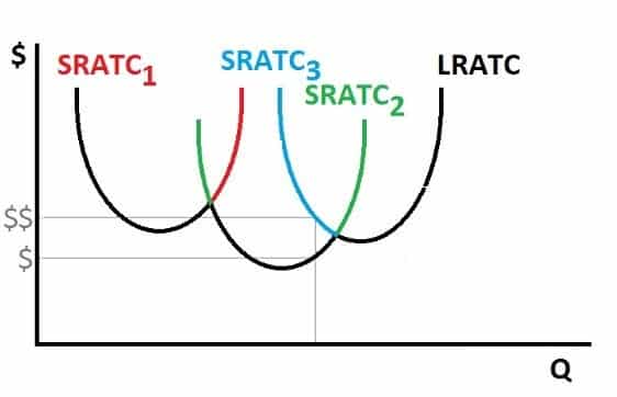
So, since each country has it’s advantages and disadvantages, and when choosing it, the costs are fixed(remember: average total costs), we start by have our first cost curve from country 1. This represents the minimum costs possible for the same quantity of output between the three countries. We state this by comparing the point of inflection in all three curves. Costs initially go down due to economies of scale(the more inputs you add the more output comes out), but then the output starts going down and costs keep going up, creating what is called diseconomies of scale.
The Long Run Average Total Cost Curve is an envelope representing the sum of all Short Run Average Total Cost Curves.
Notive the figure where its shape is marked black. It also shows the three main parts of the curve: Economies of Scale, Constant Returns to Scale and Diseconomies of Scale.

From a pur mathematical point of view, this Long Run Curve is a sum of series of discrete signals, and since we only have three, the shape is more “bumpy”. If we add much more signals, the bottom shape becomes more smooth.

The key main takeaway from this analysis is the following:
1. In the long run all costs are variable. This is not the case for the short run where lots of costs are fixed.
2. Economies of scale are achieved when the output significantly outweighs the input: 2 units of input produce 4 units of output for instance.
3. Constant returns of scale happen when the same input produces the same output: 2 units of inpout produce 2 units of output.
4. Diseconomies of scale happen when less output is achieved with more imput: 2 units of input produce less than 2 units of output.
